Visualization of chemical datasets and exploratory data analysis [Python, RDKit]

2020/2/172021/8/28

As a preliminary step to machine learning / QSAR model creation, it is important to analyze the contents of compound data consisting of a list of chemical structures and activities from a bird's-eye view in order to select and understand the model.

This time, we will perform exploratory data analysis of compound datasets as a data science method for finding features related to the objective variable.

What is exploratory data analysis?

Exploratory data analysis is an important approach in the early stages of data analysis, summarizing key features through data visualization and correlation analysis.It is done to verify whether the originally expected pattern is recognized in the data, or to look for any pattern.

1970s statistician Tukey's book "Exploratory data analysisIs now established as an important process in data analysis, with about 2 citations (Tukey, John W. Exploratory data analysis. Vol. 2. 1977.).

Data preparation

BBBP of Molecule Net is used for sample data. Regarding blood-brain barrier penetration, the data is a summary of "penetration" as XNUMX and "non-penetration" as XNUMX.

references:https://pubs.acs.org/doi/10.1021/ci300124c

Data preparation

import numpy as np
import pandas as pd
from rdkit import rdBase, Chem
from rdkit.Chem import AllChem, PandasTools, Descriptors
pd.set_option('display.max_columns',250)
print('rdkit version: ',rdBase.rdkitVersion)　#rdkit version:  2019.03.4
　
bbbp = pd.read_csv('./BBBP.csv',index_col=0)
　
# smilesからmolオブジェクトを作成し、DataFrameに格納
PandasTools.AddMoleculeColumnToFrame(bbbp,'smiles')
　
#　molオブジェクトを作れなかった行の削除
bbbp = bbbp.dropna() 
bbbp.info()

Int64Index: 2039 entries, 1 to 2053 Data columns (total 4 columns): name 2039 non-null object p_np 2039 non-null int64 smiles 2039 non-null object ROMol 2039 non-null object dtypes: int64 (1), object (3) ) memory usage: 79.6+ KB

A bird's-eye view of the dataset

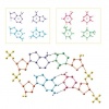
First, check the list of what kind of chemical structure is included.

#　化学構造を一覧で表示
PandasTools.FrameToGridImage(bbbp[:18], column='ROMol', legendsCol='name', molsPerRow=6, subImgSize=(150,150))

　　

# ターゲットp-npの分布を確認
bbbp.p_np.value_counts()

1 1560 0 479 Name: p_np, dtype: int64

Search for correlation with objective variable from compound descriptor

Since it is not possible to get an overview just by looking at it, create and aggregate descriptors and take a bird's-eye view of the dataset.
The compound descriptors are summarized below.

# 記述子を生成する
for i,j in Descriptors.descList:
    bbbp[i] = bbbp.ROMol.map(j)

#　要約統計量の表示
bbbp.describe()

#　データセット全体における構造記述子の分布
import matplotlib.pyplot as plt
import math

list = ["p_np", "RingCount", "NumAromaticRings", "NumAromaticCarbocycles", "NumAromaticHeterocycles", "NumSaturatedCarbocycles", "NumSaturatedHeterocycles", "NumSaturatedRings"]

fig = plt.figure(figsize=(15,7))
for i, c in enumerate(list):
   ax = fig.add_subplot(
       math.ceil(len(list) / 4), 4, i + 1)
   # plot the continent on these axes
   sns.countplot(x=c, data=bbbp,  ax=ax)
   ax.set_title(c)
fig.tight_layout()
plt.show()

　

# targetによる構造記述子の分布の違いを可視化
list = ["RingCount", "NumAromaticRings", "NumAromaticCarbocycles", "NumAromaticHeterocycles", "NumSaturatedCarbocycles", "NumSaturatedHeterocycles", "NumSaturatedRings"]
　
fig = plt.figure(figsize=(15,7))
for i, c in enumerate(list):
   ax = fig.add_subplot(
       math.ceil(len(list) / 4), 4, i + 1)
   # plot the continent on these axes
   sns.countplot(x=c, data=bbbp, ax=ax, hue="p_np")
   ax.set_title(c)
fig.tight_layout()
plt.show()

　

#　logPと分子量でplotしてみる
import seaborn as sns
sns.scatterplot(x="MolWt", y="MolLogP", data=bbbp,
                hue="p_np",
                alpha=0.5)

Since it is blood-brain barrier permeability, important factors were almost known, but it can be seen that hydrophobicity (logP) and molecular weight (MolWt) are important for membrane permeability.

The following were helpful as methods for general exploratory data analysis ( How to choose and draw the correct visualization method in exploratory data analysis ).It looks good to apply it to the aggregation of descriptors.